Image:Snells law wavefronts.gif
From Wikipedia, the free encyclopedia
No higher resolution available.
Snells_law_wavefronts.gif (225 × 227 pixels, file size: 148 KB, MIME type: image/gif)
| | This is a file from the Wikimedia Commons. The description on its description page there is shown below.
|
| Description |
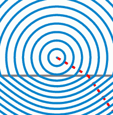
Illustration of wavefronts in the context of Snell's law. |
|---|---|
| Source |
self-made with MATLAB |
| Date |
05:36, 1 January 2008 (UTC) |
| Author | |
| Permission (Reusing this image) |
see below |
| Other versions | Image:Snells law wavefronts.png |
| I, the copyright holder of this work, hereby release it into the public domain. This applies worldwide. In case this is not legally possible: Afrikaans | Alemannisch | Aragonés | العربية | Asturianu | Български | Català | Česky | Cymraeg | Dansk | Deutsch | Eʋegbe | Ελληνικά | English | Español | Esperanto | Euskara | Estremeñu | فارسی | Français | Galego | 한국어 | हिन्दी | Hrvatski | Ido | Bahasa Indonesia | Íslenska | Italiano | עברית | Kurdî / كوردی | Latina | Lietuvių | Latviešu | Magyar | Македонски | Bahasa Melayu | Nederlands | Norsk (bokmål) | Norsk (nynorsk) | 日本語 | Polski | Português | Ripoarisch | Română | Русский | Shqip | Slovenčina | Slovenščina | Српски / Srpski | Svenska | ไทย | Tagalog | Türkçe | Українська | Tiếng Việt | Walon | 中文(简体) | 中文(繁體) | zh-yue-hant | +/- |
[edit] Source code (MATLAB)
% Illustration of Snell's law
function main()

   % indexes of refraction
   n1=1.0;
   n2=1.5;

   sign = -1;% is the source up or down?
   O=[0, -1*sign];
   k=500;


% KSmrq's colors
   red    = [0.867 0.06 0.14];
   blue   = [0, 129, 205]/256;
   green  = [0, 200,  70]/256;
   yellow = [254, 194,   0]/256;
   white = 0.99*[1, 1, 1];
   black = [0, 0, 0];
   gray = 0.5*white;

   color1=red;
   color2=blue;
   color3=gray;
   lw = 3;

   plot_line=0;
   Theta=linspace(0, 2*pi, k);
   V=0*Theta; W=0*Theta;
   S0=7;
   spacing=0.45;
   p=floor(S0/spacing);
   S=linspace(0, S0, p+1);
   spacing=S(2)-S(1);

   num_frames = 10;
   for frame_iter=1:num_frames

      figure(1); clf; hold on; axis equal; axis off;

      % plot the interface between diellectrics
      L=1.2*S0;
      plot([-L, L], [0, 0], 'color', color3, 'linewidth', lw);


      % plot a ray
      plot_line=1;
      s=L;
      theta=pi/3; wfr(s, theta, n1, n2, O, sign, plot_line, color1, lw);

      % plot the wafefronts
      plot_line=0;
      for i=1:p

         s=S(i)+spacing*(frame_iter-1)/num_frames;

         for j=1:k
            theta=Theta(j);
            [V(j), W(j)]=wfr(s, theta, n1, n2, O, sign, plot_line, color1, lw);
         end
         plot(V, W, 'color', color2, 'linewidth', lw);
      end


      %  dummy points to enlarge the bounding box
      plot(0, S0+2.5*spacing, '*', 'color', white);
      plot(0, -(S0+2.5*spacing)/n2, '*', 'color', white);

      % to know where to crop later
      Lx=3.2; Ly=Lx; shift = 1;
      plot([-Lx, Lx, Lx, -Lx -Lx], ...
           [-Ly, -Ly, Ly, Ly, -Ly]+shift);

      file = sprintf('Frame%d.eps', 1000+frame_iter);
      disp(file);
      saveas(gcf, file, 'psc2')
   end

% Converted to gif with the UNIX command
% convert -density 100 -antialias Frame10* Snell_animation.gif
% then cropped in Gimp

function [a, b]=wfr(s, theta, n1, n2, O, sign, plot_line, color1, lw);

   X=O+s*[sin(theta), sign*cos(theta)];

  if( sign*X(2) > 0 )
    t=-sign*O(2)/cos(theta);
    X0=O+t*[sin(theta), sign*cos(theta)];

    if (plot_line == 1)
      plot([O(1), X0(1)], [O(2), X0(2)], 'color', color1, 'linewidth', lw, 'linestyle', '--');
    end

    d = norm(O-X0);
    r = (s-d)*(n2/n1)^(sign);

    theta2=asin(n1*sin(theta)/n2);
    XE=X0+r*[sin(theta2), sign*cos(theta2)];
  else
    XE = X;
  end
  a = XE(1);
  b = XE(2);

  if (plot_line==1)
    plot([X0(1), XE(1)], [X0(2), XE(2)], 'color', color1, 'linewidth', lw, 'linestyle', '--');
  end
File history
Click on a date/time to view the file as it appeared at that time.
| Date/Time | Dimensions | User | Comment | |
|---|---|---|---|---|
| current | 06:31, 2 January 2008 | 225×227 (148 KB) | Oleg Alexandrov | ({{Information |Description=Illustration of wavefronts in the context of Snell's law. |Source=self-made with MATLAB |Date=05:36, 1 January 2008 (UTC) |Author= Oleg Alexandrov |Permission= |oth) |

