Image:Double torus illustration.png
From Wikipedia, the free encyclopedia
Size of this preview: 569 × 600 pixels
Full resolution (1,176 × 1,240 pixels, file size: 350 KB, MIME type: image/png)
| | This is a file from the Wikimedia Commons. The description on its description page there is shown below.
|
| Description |
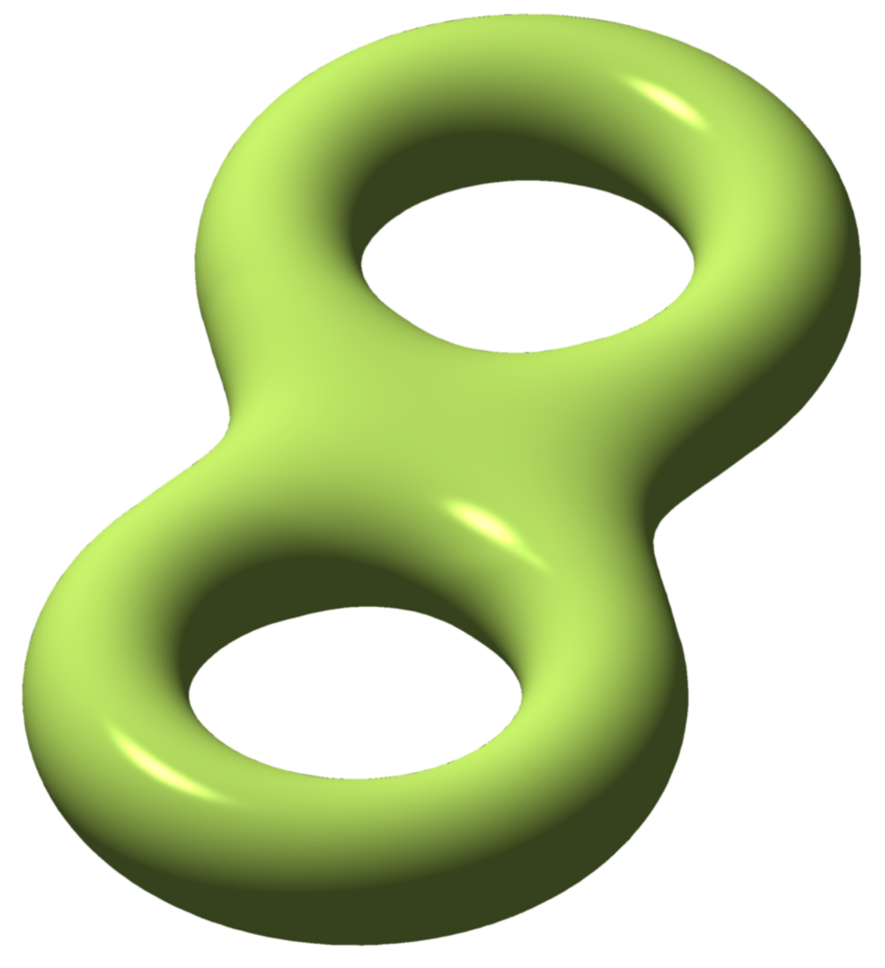
Illustration of en:Double torus |
|---|---|
| Source |
self-made |
| Date |
05:50, 6 September 2007 (UTC) |
| Author | |
| Permission (Reusing this image) |
see below |
| I, the copyright holder of this work, hereby release it into the public domain. This applies worldwide. In case this is not legally possible: Afrikaans | Alemannisch | Aragonés | العربية | Asturianu | Български | Català | Česky | Cymraeg | Dansk | Deutsch | Eʋegbe | Ελληνικά | English | Español | Esperanto | Euskara | Estremeñu | فارسی | Français | Galego | 한국어 | हिन्दी | Hrvatski | Ido | Bahasa Indonesia | Íslenska | Italiano | עברית | Kurdî / كوردی | Latina | Lietuvių | Latviešu | Magyar | Македонски | Bahasa Melayu | Nederlands | Norsk (bokmål) | Norsk (nynorsk) | 日本語 | Polski | Português | Ripoarisch | Română | Русский | Shqip | Slovenčina | Slovenščina | Српски / Srpski | Svenska | ไทย | Tagalog | Türkçe | Українська | Tiếng Việt | Walon | 中文(简体) | 中文(繁體) | zh-yue-hant | +/- |
[edit] Source code
% illustration of a double torus
function main()

   % N = The number of data points. More points means prettier picture.
   N=100;

   % big and small radii of the torus
   R = 3; r = 1;

   % c controls the transition from one ring to the other
   c = 1.3*pi/2;

   Kb = R+r;
   Ks = R-r;

   % plot the two rings
   Ttheta=linspace(0, 2*pi, N);
   Pphi=linspace(0, 2*pi, N);
   [Theta, Phi] = meshgrid(Ttheta, Pphi);
   X=(R+r*cos(Theta)).*cos(Phi);
   Y=(R+r*cos(Theta)).*sin(Phi);
   Z=r*sin(Theta);

   figure(4); clf; hold on; axis equal; axis off;
   axis([-Kb 3*Kb -Kb Kb -r r]);
   light_green=[184, 224, 98]/256; % light green
   myplot(X, Y, Z, light_green);
   myplot(X+2*Kb, Y, Z, light_green);

% Plot the "waist" joining the two rings. This is the hardest.
% All the code below is devoted to that. It is just a hack

%  Dirty tricks to get a grid more adapted to the torus geometry
   N1 = N; N2 = N; N3 = N1;
   N4 = N1;
   small = 0.3*r;
   tiny = 0.001;

   % plot the "waist" of the torus
   XX = linspace(R-r, R+3*r, 4*N);
   YY=linspace(-Kb, Kb, N);
   [X, Y] = meshgrid(XX, YY);

   % Modify Y to make it more adapted to the torus geometry
   M = length(XX);
   for j=1:M
      x = XX(j); x = my_map(x, Kb, c);
      bl = sqrt(Kb^2-x^2);
      bm = sqrt(max(Ks^2-x^2, 0));

      k = 10; tiny = 1/N;
      Y1 = linspace(-bl, -bm, N/2-k); % Y1=adaptive_grid(Y1);
      Y2 = linspace(-bm+tiny, bm-tiny, 2*k); %Y2=adaptive_grid(Y2);
      Y3 = linspace(bm, bl, N/2-k);  %  Y3 = adaptive_grid(Y3);

      Y(:, j)=[Y1 Y2 Y3]';
   end

   [m, n] = size(X);
   for i=1:m
      for j=1:n

         x = X(i, j); x = my_map(x, Kb, c);
         y = Y(i, j);

         z = r^2 - (sqrt(x^2+y^2)-R).^2;
         if z < 0
            z = NaN;
         else
            z = sqrt(z);
         end

         Z(i, j) = z;
      end
   end


   myplot(X, Y, Z, light_green);
   myplot(X, Y, -Z, light_green);


% viewing angle
   view(108, 42);

% add in a source of light
   camlight (-50, 54); lighting phong;

% save as png
%  print('-dpng', '-r300', sprintf('Double_torus_illustration_N%d.png', N));

function myplot(X, Y, Z, mycolor)

   H=surf(X, Y, Z);

   % set some propeties
   set(H, 'FaceColor', mycolor, 'EdgeColor','none', 'FaceAlpha', 1);
   set(H, 'SpecularColorReflectance', 0.1, 'DiffuseStrength', 0.8);
   set(H, 'FaceLighting', 'phong', 'AmbientStrength', 0.3);
   set(H, 'SpecularExponent', 108);

% This function constructs the second ring in the double torus
% by mapping from the first one.
function y=my_map(x, K, c)

   if x > K
      x = 2*K - x;
   end

   if x < K-c
      y = x;
   else
      y = (K-c) + sin((x - (K-c))*(pi/2/c));
   end


% take a uniform grid and cluster its points toward the endpoints
function X = adaptive_grid (X)

   K = 50;

   n = length(X);
   a = X(1); b = X(n);


   if a == b
      return;
   end

   X = (X-a)/(b-a);
   X = atan(K*(X-0.5));

   X = (X-X(1))/(X(n)-X(1));
   X = a + (b-a)*X;
File history
Click on a date/time to view the file as it appeared at that time.
| Date/Time | Dimensions | User | Comment | |
|---|---|---|---|---|
| current | 05:49, 6 September 2007 | 1,176×1,240 (350 KB) | Oleg Alexandrov | ({{Information |Description= |Source=self-made |Date=Illustration of en:Double torus |Author= Oleg Alexandrov }} {{PD-self}} Category:Differential geometry Category:Files by User:Oleg Alexandrov from en.wikipedia) |

